The power sources most familiar for the supply of renewable energy – wind, sun and water – are considered to be freely available; therefore a common assumption is that the energy provided by these power sources is also free. A stand-alone power system (SAPS), in order to take advantage of ‘free’ energy sources, costs money to establish, to operate and to maintain/replace equipment in the future. The cost of the system’s power equipment, e.g. PV modules, the inverter, the batteries, the installation and balance of system (BOS) equipment can be significant. In essence you are paying for ‘X’ years of energy up front and then utilising “free” energy resources, subject to their prevailing availability.

Conversely, energy from non-renewable energy sources (diesel, natural gas, LP gas etc.) is not free (i.e. you need to continually buy fuel), but the cost of establishing a system to use these energy sources for SAPS is generally less than the system costs for a renewable energy SAPS.

A SAPS is thus a financial investment: it involves costs, both upfront and ongoing, and provides benefits in return. To be able to make an informed decision about whether to invest in a SAPS, an economic analysis should be performed. In some cases, the installation of a SAPS may be necessary regardless of cost; in this case a financial analysis comparing multiple design options (e.g. predominately PV generation versus a diesel-only system) will be of great benefit.

Typically the analysis is performed to compare the options available to assist in decision making and these will be site and resource specific.

To perform a lifetime economic analysis of the options, initial capital costs and operating costs need to be determined. These include:

• Capital expenditure (CAPEX): The total cost to set up an option. Financial arrangements might mean that the initial upfront cost is replaced with regular ongoing contractual payments.
• Rebates: Any technology allowances, grants, rebates or financial discounts available at the time of the initial purchase.
• Operational expenditure (OPEX): Any future costs associated with the system, such as fuel costs, maintenance costs and component replacement. These may include rebates that reduce OPEX.

Life cycle cost analysis

Life cycle cost analysis is a relatively complex economic analysis of SAPS, but due to the methods used, it is the only way to fairly and accurately compare options. Whilst the formulae may seem complex, spreadsheets have these functions ‘built in’ and greatly simplify the process.

The basic premise is that it takes into account that the value of money varies over time, both in the interest accrued by money not spent and in inflation, which reduces the spending value of money. This is particularly important for any future costs and benefits, such as maintenance costs or product replacements.

As the value of money spent or earned in the future changes depending on when it is spent or earned, all future costs and incomes are brought back to their ‘present day value’. This allows comparisons to be made between systems that will have different costs at different times in the present and the future.

To bring costs and incomes to their present day value, two terms are used to adjust the value of money spent in the future:

• Inflation rate: Money loses value over time owing to the inflation of the value of goods and services. This means the spending power decreases over time. For example, a meal might cost $10 today but inflation will reduce the spending power of money over time so after 10 years the same meal’s cost may be $15.
• Discount rate: The discount (or interest) rate represents the amount at which unspent money grows due to accrued interest. For example, the value of $100 spent now will be less than the end value of $100 that has been saved and accrued interest for a period of 10 years. Therefore, any calculation of the future cost of that investment must take into account the fact that spending the money meant that it could not accrue interest in a bank.

As can be seen, the inflation rate decreases the value of money over time, whereas the discount rate increases the value of money over time.

Rather than include inflation, accepted practice, particularly in government procedures for “value for money” analysis is to use a ‘real’ discount rate. These rates reflect the real (after inflation) rates of return these sectors could normally expect to achieve on low-risk investments. Government agencies and donor entities usually have a set discount rate to be used for comparing options.
The choice of discount rate affects the life cycle cost of a PV system substantially since these systems have high capital costs and low running costs. Therefore, the economic and social benefits accrue over the life of the system.
It is often useful to examine the sensitivity of the costing in relation to changes in discount rate. Again, government agencies and donor entities will usually specify the discount rates to be used in sensitivity analysis.

Life cycle costs

Life cycle cost takes the following into consideration:

• The initial cost of all the equipment and installation and commissioning labour.
• The future cost of all operation and maintenance, adjusted for the time value of money.
• The future cost of all component replacements, adjusted for the expected time of replacement.
• The future cost of end-of-life disposal or recycling.
• It is extremely important to use best available information and not be tempted to use data that favours a particular option, that for non-economic reasons may be the preferred option. This latter choice can be made after analysing life cycle costs on an equitable basis.

Present Day Value of Future Costs

Any future costs need to consider that the value of money changes over time. These future costs can be converted into a present day value using the following formula:

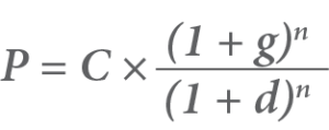
Where:

• P = The present value of the future cost.
• C = The future cost.
• g = The inflation rate.
• d = The discount (interest) rate.
• n = The number of years in the future.

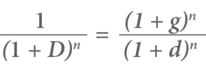
Again, accepted practice is that costs and benefits should be valued in ‘real’ terms: that is they should be expressed in constant money (e.g. dollars) and increases in prices due to the general rate of inflation should not be included in the values placed on future benefits and costs. A ‘real’ discount rate, D, can replace the inflation and interest rates in the previous equation:

In this case the formula for present day value can be written simply as:

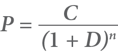
Where:

• P = The present value of the future cost.
• C = The future cost in real terms.
• D = The ‘real’ discount rate.
• n = The number of years in the future.

The stream of costs and benefits (expressed in real terms) should be discounted by the ‘real’ discount rate, say 7%, with sensitivity analysis using discount rates of 4% and 10%.

For example

• If the maintenance cost is $500 in the first year, this is the value used for all subsequent years, which are then discounted to today’s value.
• If today’s cost of replacing an inverter is $5,000, then in whatever year (year n) it is expected to be replaced, then the cost is also entered as $5,000, then discounted using the above formula for year n.
• An exception to the ‘real’ cost being different in the future is when a component’s current cost is expected to reduce due to factors such as technological and manufacturing developments or even economies of scale. An example is lithium ion batteries that are forecast to reduce in real (today’s) cost over time.

Life Cost Example

This example calculates the life cycle cost for a SAPS with a 10kWp PV array, battery bank and inverter over a period of 20 years, using the following information:

• Initial components cost = $22,000
• Initial installation cost = $8,000
• Annual maintenance (at end of year) = $500
• Inverter and battery replacement (including disposal) at 10 years = $12,000
• ‘Real’ discount rate = 7%
• Disposal fees for batteries at 20 years = $1,000

Using the present day value formula, the lifetime costs have been calculated as follows

Year	Installed system		Part Replacement		System Maintenance
	Unit cost	Present day value	Unit cost	Present day value	Unit cost	Present day value
0	$30,000	$30,000
1					$500	$467
2					$500	$437
3					$500	$408
4					$500	$381
5					$500	$356
6					$500	$333
7					$500	$311
8					$500	$291
9					$500	$272
10			$12,000	$6,100	$500	$254
11					$500	$238
12					$500	$222
13					$500	$207
14					$500	$194
15					$500	$181
16					$500	$169
17					$500	$158
18					$500	$148
19					$500	$138
20			$1000	$258	$0	$0
Total		$30,000		$6,358		$5,165
Life cycle cost is the grand total of present day cost						$41,523

Levelised cost of electricity

The levelised cost of electricity (LCoE) indicates the cost of producing energy using a particular generation source and thus provides an equitable method for comparing generation options. It uses the life cycle cost of the generator, being the upfront cost and the running costs, as well as the expected yield (energy generated) over the lifetime of the generator.

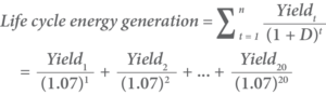
To perform an accurate LCoE calculation, any future yields (generation) from the generator must also be adjusted to their present day value.. In any year the value would be the yield for that year multiplied by the unit value for that year. As the financial value of the yields are not known at this point, the known yield is discounted to account for this.

Hence, the formula for calculating LCoE is:

More accurately, this can be written as:

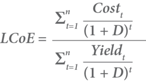
Where:

• ∑ = Sum (i.e. calculate values for each year between t and n and then add them all together).
• Cost_t = The future cost for year t.
• Yield_t = The future energy yield for year t.
• t = The year.
• D = The discount rate.
• n = The life of the system.

Levelised cost of electricity example

The LCoE of the 10 kW SAPS PV system is to be calculated over a 20 year period.

The life cycle cost has already been calculated to be $41,523.

The life cycle energy yield now needs to be calculated.

For this calculation, it is assumed that the annual system yield is 20,000 kWh but that there is a 1% decrease in the system yield each year due to the natural degradation of the system. Also:

• Discount rate = 7%

Using the following formula the energy yield is calculated as shown in below

Year	Generation with 1% drop (kWh)	Present day value (kWh)
1	19,800	18,505
2	19,600	17,119
3	19,400	15,836
4	19,200	14,648
5	19,000	13,547
6	18,800	12,527
7	18,600	11,583
8	18,400	10,709
9	18,200	9,900
10	18,000	9,150
11	17,800	8,457
12	17,600	7,815
13	17,400	7,220
14	17,200	6,670
15	17,000	6,162
16	16,800	5,691
17	16,600	5,255
18	16,400	4,852
19	16,200	4,479
20	16,000	4,135
Life cycle energy generation (kWh)		194,260

Using the following formula, the LCoE can be calculated:

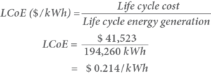
Thus, this system generates electricity at a cost of 21.4 c per kWh.

For sensitivity analysis:

A discount rate of 4% results in a LCoE of 18.3 c per kWh.

A discount rate of 10% results in a LCoE of 24.7 c per kWh.

The LCoE is used to compare the average cost of electricity from different generation sources. For example if the same annual energy is to be supplied by a diesel genset. In this case there is more maintenance to be included as run hours determines the type of maintenance and associated costs. The calculations of the genset option are not shown in this extract, but the comparison between PV and genset options are shown in the following table.

The LCoE calculations and sensitivity analysis show that the PV SAPS is cheaper in all cases. They also highlight that lower discount rates favour a SAPS with higher capital costs and lower operating costs, whilst higher discount rates improve the lower capital cost system with higher operating and future replacement costs.

Discount rate	PV SAPS cents per kWh	Genset SAPS cents per kWh
4%	18.3	53.0
7%	21.4	41.5
10%	24.7	33.5

This is an extract from the Economics Chapter of Version 8 of the GSES Stand Alone Power Systems publication, a forthcoming definitive publication within the Renewables industry.